In which we train an TensorFlow model with the tears of my little one, then deploy it on a Raspberry Pi.

The last time we met, we had a lively discussion about the ins and outs and joys and terrors of parenting. I talked about how I started building a Raspberry Pi project with a USB mic and wrote a simple parsing script that measured the mean amplitude of recordings of the current state of the nursery. And when that guy wailed, he really WAILED.

Well that naive approach got us so far, but the system would still trip up due to random loud noises in the house. Music, or doors closing or opening, or loud conversation would all cause the system to think the kid was crying but no - it was just ambient noise.

Getting started with TensorFlow

Let’s start our dive into machine learning!

I had already gotten pretty far with Udacity’s Machine Learning course and had vague recollections of AI theory floating around from the cobwebs of undergrad CS courses past. So I had some background in AI and machine learning. But training neural networks was a completely new thing to me.

Luckily, I came across the Simple Audio Recognition Tutorial example right there on the TF homepage. This was exactly what I was looking for. The objective was: given a training set of audio clips of crying babies and “empty rooms”, classify an audio clip as one or the other.

First: getting the dataset

I had oversimplified in my mind what made a great training data set. After all, I figured that I just had to record my kid crying a bunch, then get a few minutes of quiet room sounds, and then we were good, right?

Wrong.

Training data must be exactly matched. Sample rates must be consistent, and audio samples must either be highly randomized or at least normalized to the same rates. To wit, here’s how I gathered my sample data:

1. I set up the Raspberry Pi to continuously record 30-second samples at 22.05kHz through the onboard microphone.
2. When my son started a crying episode, I’d make note of the start time and end times, and then go back and gather those clips of the cries and dump them in the crying folder.
3. Once I had collected enough of those (maybe 30 minutes total), I then gathered a bunch of the “other” clips of quiet sleep in his nursery and threw these in the silence folder.
4. Once I had moved these samples off the Raspberry Pi and onto my laptop, I then sliced these recordings into 5-second clips using sox. I also applied a few amplification filters to overcome the weak pickup on the mic.

$ sox FILENAME FILENAME_OUTPUT trim 0 5 vol 45 dB rate 22050

I then placed each of these trained samples in the folders corresponding to their label: crying and silence.

Second: training the network

I modified the train.py script nearly verbatim from TF docs. We’ll dissect it here, beginning with the command to begin training:

1
    $ python app/train.py --data_url= --data_dir=./data --wanted_words=silence,crying --sample_rate=22050 --clip_duration_ms=5000 --how_many_training_steps=1000,200 --learning_rate=0.001,0.0001 --train_dir=./training

• --wanted_words=silence,crying: This specifies which labels should be considered for training purposes.
• --sample_rate: The sample rate of the audio files provided
• --clip_duration_ms: Duration of each training clip in milliseconds
• --how_many_training_steps: This is a comma-separated list of n numbers that specify the number of steps per phase.
• --learning_rate: This is the rate at which the system can adjust its current learnings to match its new inputs. A higher learning rate means the faster the system can change to learn new inputs. A lower number ensures the stability of a system’s learning. We specify a higher training rate for the first phase and lower the training rate in the latter phase as our precision increases.

Let’s run the script!

1
2
3
4
5
6
7
8
9
$ python app/train.py --data_url= --data_dir=./data --wanted_words=silence,crying --sample_rate=22050 --clip_duration_ms=5000 --how_many_training_steps=1000,200 --train_dir=./training
2018-08-27 22:15:33.195894: I tensorflow/core/platform/cpu_feature_guard.cc:140] Your CPU supports instructions that this TensorFlow binary was not compiled to use: AVX2 FMA
Tensor("Placeholder:0", shape=(), dtype=string)
INFO:tensorflow:Training from step: 1
INFO:tensorflow:Step #1: rate 0.001000, accuracy 26.0%, cross entropy 2.674081
INFO:tensorflow:Step #2: rate 0.001000, accuracy 23.0%, cross entropy 1.593786
INFO:tensorflow:Step #3: rate 0.001000, accuracy 64.0%, cross entropy 1.067298
INFO:tensorflow:Step #4: rate 0.001000, accuracy 73.0%, cross entropy 0.843605
...

Third: parsing the results

The output in each step reveals the current state of the neural network as trained. Accuracy reflects the correctness of the model as the validation set is tested against the network (during each step of training, samples in the validation set are run against the model and checked if they line up with their specified labels).

Cross entropy is, as I understand it, the squared error factor in the result network from the actual results (lower is better).

This would proceed for several hours for 1200 total steps. On a 2013-era Macbook Pro, this took approximately 6 hours. I had 350 clips of crying and 500 clips of silence. (Too much or not enough? This tired parent says “too much”.)

One more thing - every few hundred steps during training, we would get this sort of output:

1
2
3
4
5
INFO:tensorflow:Confusion Matrix:
 [[ 9  0  0  0]
 [ 0  0  0  0]
 [ 0  0 55  0]
 [ 0  0  1 30]]

What’s a confusion matrix? It’s, according to this helpful article, another way to visualize the accuracy of a machine learning model.

Here’s how to read this confusion matrix. Given the following labels:

1
2
3
4
5
# conv_labels.txt
_silence_
_unknown_
silence
crying

(Where did these come from? More on that later…)

Imagine these labels go left-to-right, and top-to-bottom. The x-axis represents the labels that have been predicted (i.e. that have been verified) to be a certain label. So the first column represents the percentages of samples that have been predicted to be _silence_.

The labels that go top-to-bottom are the actual results from the trained model. So in this case, if we take the top-left number 9, that means that in 9 runs of the model where the prediction was _silence_, the actual result was _silence_. Moving one cell down, that represents the # of samples where the predicted result was _silence_, but the actual result was _unknown_. Fortunately for our model, there are 0 results in this cell. So on and so forth. So the ideal confusion matrix is a matrix that has a “diagonal line” running from top-left to bottom-right, and 0s everywhere else, because all predictions would equal actuals.

tl;dr: Confusion matrices are a way to visualize and report the accuracy of a machine learning model. You want a clear and convincing diagonal line in the matrix.

Oh, and here are the results from the training data. I’m using tensorboard to visualize the training steps:

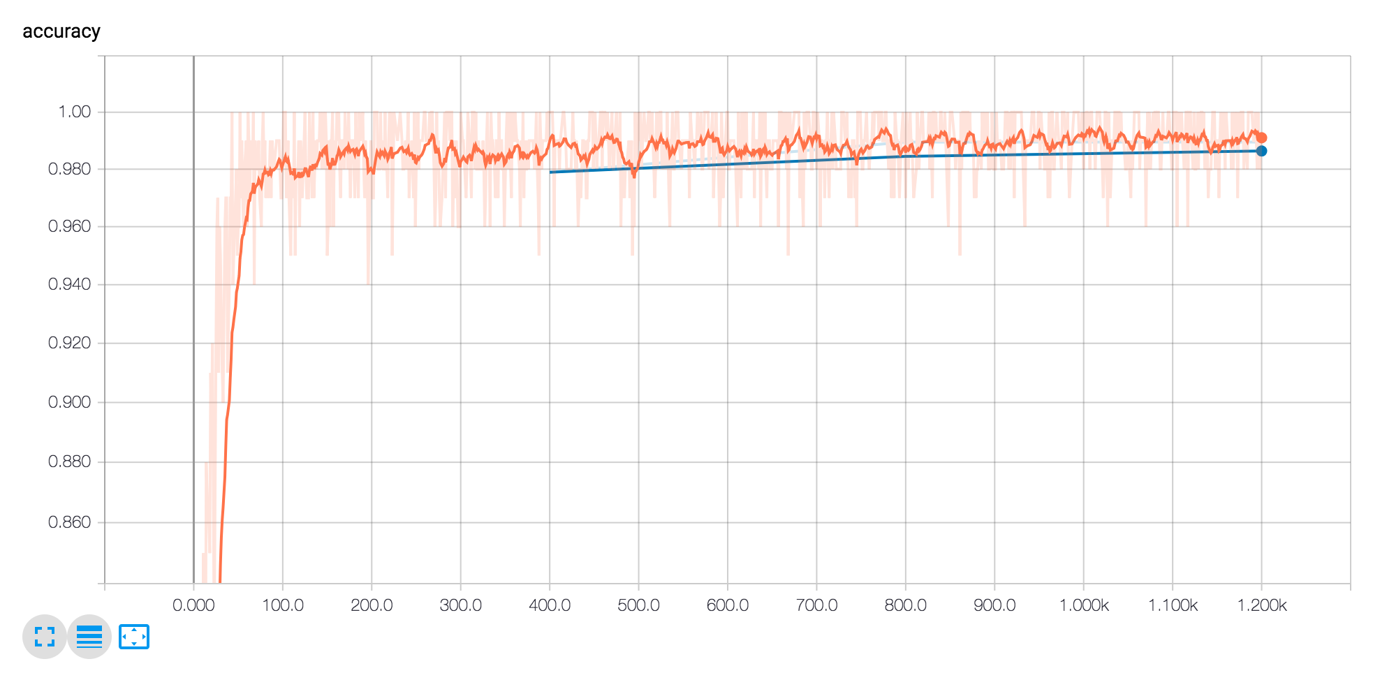Accuracy modeling. Note how quickly the model jumps to be fairly accurate.

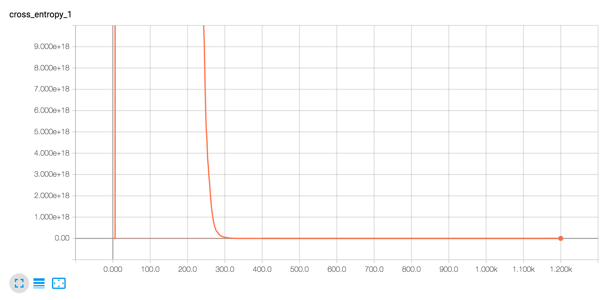Note how quickly cross entropy dives.

We can use these graphs to tune our models if we really cared. In this case, I say it’s good enough (accuracy is up to 99% by the end).

Fourth: Saving and exporting the model

OK, but enough already. We have a trained model and, like Chekhov’s Gun, that means we’ve gotta use it!

Where’s that model? Oh, it needs a few more steps before it can emerge. At this point, TensorFlow has developed a neural network, but the neuron graph (is that the right term?) is not yet in a usable state to be used by applications. To that point, we need to dump the model into a binary format that can be used by TensorFlow applications in the future.

Once again, I claim no smarts in all this, but instead point to the TensorFlow script to do this in app/freeze.py:

1
$ python app/freeze.py --start_checkpoint=./training/conv.ckpt-1200 --output_file=./graph.pb --clip_duration_ms=5000 --sample_rate=22050 --wanted_words=silence,crying --data_dir=./data

What did we specify here?

We said we wanted the model at --start_checkpoint of 1200, saving the --output_file to graph.pb, and mentioning that the sample rate of each audio sample should be 22050 hz and 5 seconds long. We then specified that the labels we wanted to classify are silence and crying. Finally, the data set from the prior run can be found in ./data dir.

When we run this script, we get a graph.pb protobuf binary file that we can then ship to various TensorFlow programs.

Fifth: Using the model

Now here’s the fun part!

Onboard a Raspberry Pi, we are now going to play back current samples in the nursery:

Every 1 minute (with cron), we record audio samples from the system mic in the baby’s nursery. We then massage, crop and downsample it into a WAV file. We then point a script at this WAV file and run the TF graph on it. Running the graph will return a list of labels and their probabilities. We choose the first label with the highest probability, and ship it off to a timeseries API, in this case powered by Keen.io.

Voila:

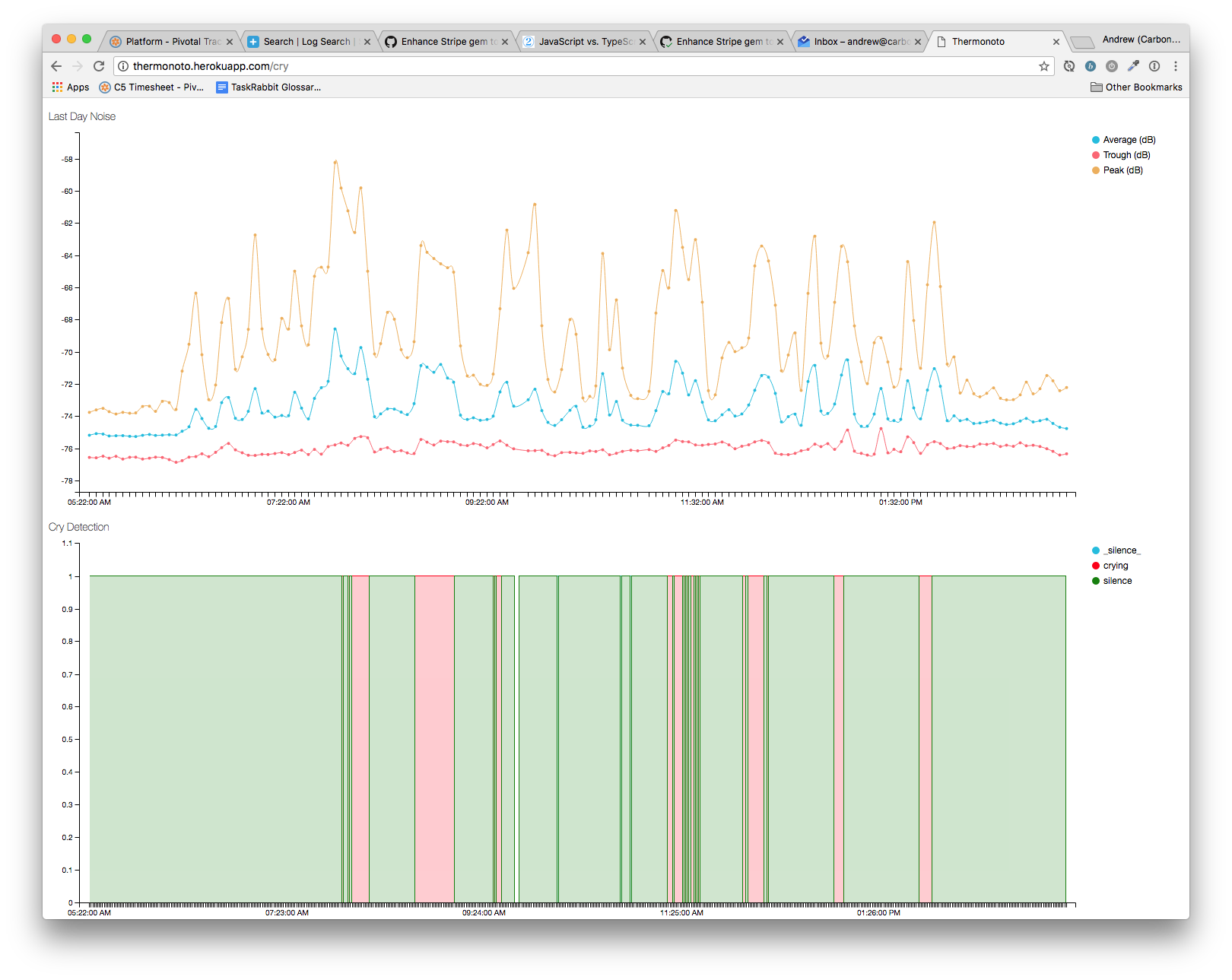A fun graph displaying the timeseries data for this little dude’s episodes. On the top was the original RMS volume graph, and the bottom is the result of the trained TF model. Note how much easier to read and understand the latter graph is.

Show me the code!

Much of this code has been adapted from Google’s TensorFlow Audio Recognition tutorial.

My scripts have been collected on this GitHub repository: https://github.com/andrewhao/babblefish

And my repository with audio sampling and archiving: https://github.com/andrewhao/miserymeter

Conclusion

Wow, that was a quick dive through TensorFlow. Note that I didn’t get too deep into the theory of convolutional neural networks, which may be a topic of discussion for another time. Instead, we talked a little bit about the mechanics of building and training a TF model with audio data and a finite set of classes. It was fairly straightforward to get this script then loaded up on a Raspberry Pi and have a dashboard that could finally quantify the pain and suffering of baby… and parent.

Epilogue

The months that went into developing this app were fully and knowingly an escape from the very real stressors of parent life. I want to acknowledge the love, the grit and the patience of my wife in this very trying time. There is so much more to say about babies other than their crying and fussing - life these days is filled with laughter and giggles and joy, too - but these are words that I’ll save for another blog entry on a different blog for another time.